Chapter Notes: Introduction to Linear Polynomials

1. Introduction

Welcome to the intriguing world of polynomials! These mathematical expressions, made up of numbers and variables, are essential in algebra and help us model real-life situations.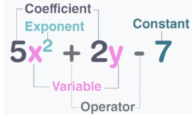 

Term	Meaning	Example
Coefficient	The number multiplied by a variable.	5 (for x2) and 2 (for y)
Variable	A symbol (usually a letter) representing a value.	x and y
Exponent	A number showing how many times to multiply the base by itself.	2
Operator	The symbol that shows the operation (addition, subtraction, etc.).	+ and –
Constant	A number that remains fixed and has no variable attached.	7

Use of Algebra in Real Life

Algebra is used in real life to solve everyday problems easily. It helps in calculating quantities, costs, and measurements using variables and expressions instead of repeated calculations. This makes work faster and more efficient in areas like shopping, construction, and science.

Example:A fruit seller packs apples and oranges. Each apple box has 10 apples and each orange box has 12 oranges. If a customer buys x apple boxes and y orange boxes and gets 5 extra fruits free, find the total number of fruits.

Ans: Each apple box → 10 apples → x boxes give 10x apples
Each orange box → 12 oranges → y boxes give 12y oranges
Extra fruits = 5
So, total = 10x + 12y + 5
Example: A rope of length 24 m is used to form a rectangle. Let the width be x m.Find the area of the rectangle.
Ans: Total rope = perimeter = 24 m
So, 2(length + width) = 24 → length + width = 12
If width = x, length = (12 – x)
Area = length × width = x(12 – x) = 12x – x²

Univariate Polynomials

Algebraic expressions in one variable involving that variable raised to non-negative integer powers are called univariate polynomials (or simply polynomials).
The degree of a polynomial = the highest power of the variable.

Type	Degree	Example
Constant Polynomial	0	8 (= 8x0)
Linear Polynomial	1	3z + 7
Quadratic Polynomial	2	x2 + 5x + 1
Cubic Polynomial	3	5y3 + y2 + 2y – 1

All these have only one variable, so they are called univariate polynomials.

2. Linear Polynomials

A linear polynomial is an expression of the form $ax+b$, where a ≠ 0.

Key properties:

• When a linear polynomial is equated to a constant, we get a linear equation.
• Linear polynomials can be viewed as input-output (function) machines: for every value of x, there is exactly one output value.
• The difference between successive values at consecutive integers is constant.

Example : 
1. A gym charges a registration fee of ₹500 and ₹100 per day for using its facilities.

Days (x)	0	1	2	3	4
Amount (₹)	500	___	___	___	___

2. Write a linear equation to represent the total amount $y$y in terms of the number of days $x$x.

Ans:

Days (x)	0	1	2	3	4
Amount (₹)	500	600	700	800	900

2. Total amount = fixed fee + (cost per day × number of days)
y= 100x + 500

This is a linear polynomial in x. The amount increases by a constant ₹100 for every additional day.

3. Exploring linear patterns

A linear pattern is a sequence of numbers where the difference between any two consecutive terms is constant.

Example: The growing pattern of square tiles produces the sequence 1, 3, 5, 7, 9, … with a constant difference of 2.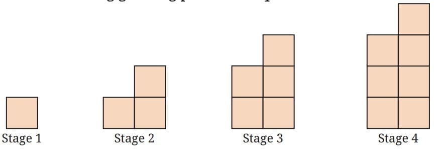

Each stage is obtained by adding two more tiles to the previous stage.The table mentions the number of tiles for the first seven stages.

General term (number of tiles at stage n):$$T_n=2n-1$$

The polynomial 2n – 1 has degree 1, confirming this is a linear pattern.

Example: A bus fare is ₹30 for the first 3 km. After that, it increases by ₹10 per km.

What will be the total fare for a journey of 12 km?

Ans: For the initial 3 km, the fare is ₹30. For every kilometre (km) thereafter, the fare will increase by ₹10. Therefore, the total fare for a travel of 12 km will be ₹30 + 10 × 9 = ₹120.

Km travelled	1	2	3	4	5	6
Fare (₹)	30	30	30	30 + 1 × 10 = 40	30 + 2 × 10 = 50	30 + 3 × 10 = 60

Total fare for a travel of n km will be ₹30 + 10 × (n – 3) = 10n, when n ≥ 3. Here, the fare for a specific distance covered is a function of the distance n km.

The slope of the linear relationship equals the constant difference between consecutive terms.

4. Linear Growth and Linear Decay

Concept	Description	Graph Slope
Linear Growth	Quantity increases by a fixed amount over equal intervals	Positive (+)
Linear Decay	Quantity decreases by a fixed amount over equal intervals	Negative (-)

Example: The temperature of a liquid is 80°C at the start of an experiment. The temperature $T$T (in °C) after $t$t minutes is given by the linear function

$T\left(t\right)=80–2t$

Time (t, minutes)	0	1	2	3	4
Temperature (°C)	80	78	76	74	72

Each minute, the temperature decreases by 2°C → Linear Decay

5. Linear Relationships

A linear relationship between two variables x and y is expressed as:
$$y=ax+b$$
where a is the slope and b is the y-intercept.
To find a and b, substitute two known (x, y) pairs and solve the resulting system of equations.

Example: A taxi service charges a fixed fee plus a cost per kilometre.
Given:
5 km → ₹120
15 km → ₹320

Find a and b in y = ax + b

Ans:

Substitute values:
120 = 5a + b
320 = 15a + b

Subtract equations:
320 – 120 = (15a + b) – (5a + b)
200 = 10a → a = 20

Put in first equation:
b = 120 – 5×20 = 120 – 100 = 20

So, y = 20x + 20 represents the fare.

6. Visualising Linear Relationships

1. Linear Equation as a Straight Line
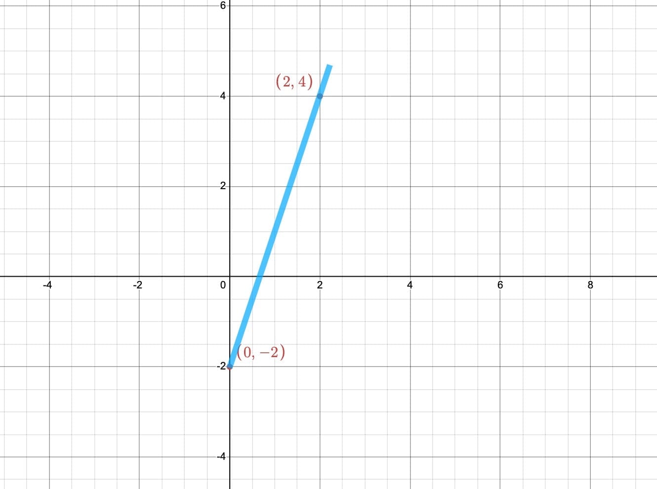
A linear relationship is written as y = ax + b. To draw its graph, we find at least two points that satisfy the equation and plot them on a coordinate plane. Joining these points gives a straight line.

Example:For y = 3x – 2, when x = 0, y = -2 → (0, -2), and when x = 2, y = 4 → (2, 4). Plot and join these points.

Ans: It gives a straight line

2. Points on a Line

A point lies on a line only if its coordinates satisfy the equation.
Example: For  y = 3x – 2, point (2,4) lies on the line because 4= 3(2)-2

3. Finding Equation from Points
If several plotted points lie on a straight line, we can find the equation by observing the pattern between x and y.

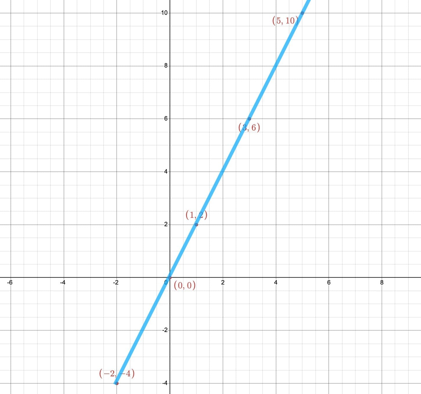
Example:Plot the points (-2, -4), (0, 0), (1, 2), (3, 6), (5, 10) on the coordinate plane. Join the points (-2, -4) and (5, 10) using a ruler.

Observe that all the points lie on a straight line. Can you find the equation of this line by identifying the relationship between x and y?

In each case, y is 2 times x

So, the equation of the line is: y= 2

4. Slope of a Line
In the equation y = ax, the number a is called the slope. It shows how steep the line is. All such lines pass through the origin (0, 0).
Example: For y = 2x, slope = 2, so the line rises faster than y = x.
5. Positive and Negative Slope
If slope (a) is positive, the line goes upward (left to right) → linear growth.
If slope is negative, the line goes downward → linear decay.

Example: y = -2x has negative slope, so the line slopes downward.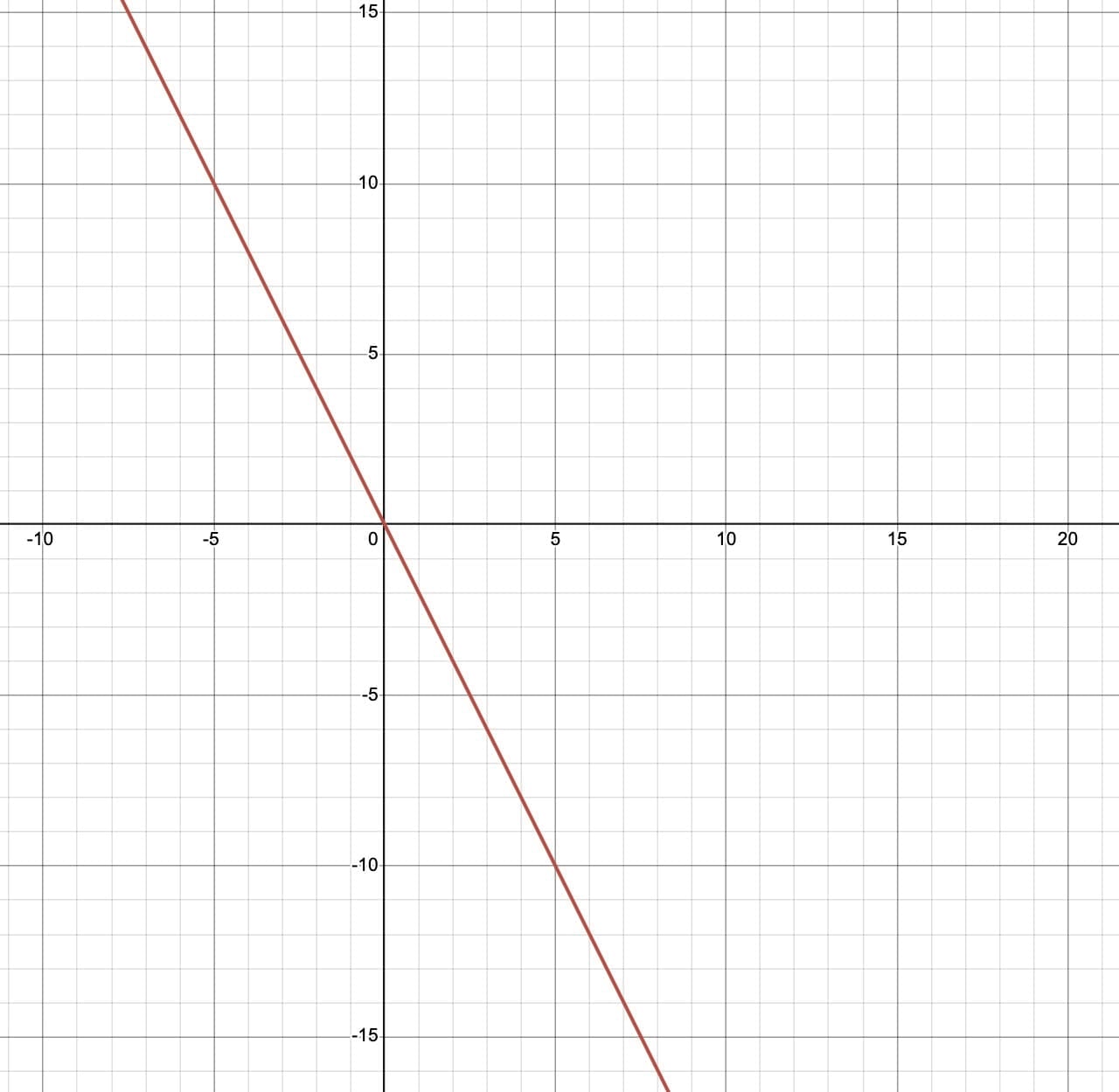6. Effect of Changing Slope (a)
When a increases, the line becomes steeper. When a decreases, the line becomes less steep.
Example: y = 3x is steeper than y = x.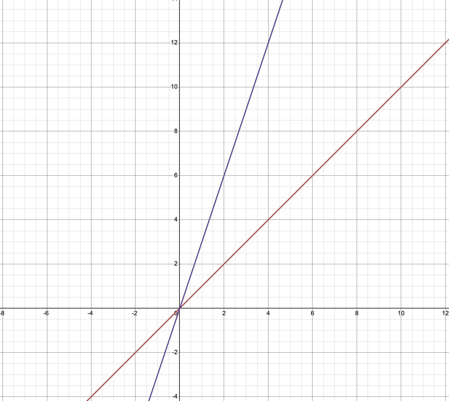Purple y=3x
Red y= x

7. Effect of Changing Intercept (b)
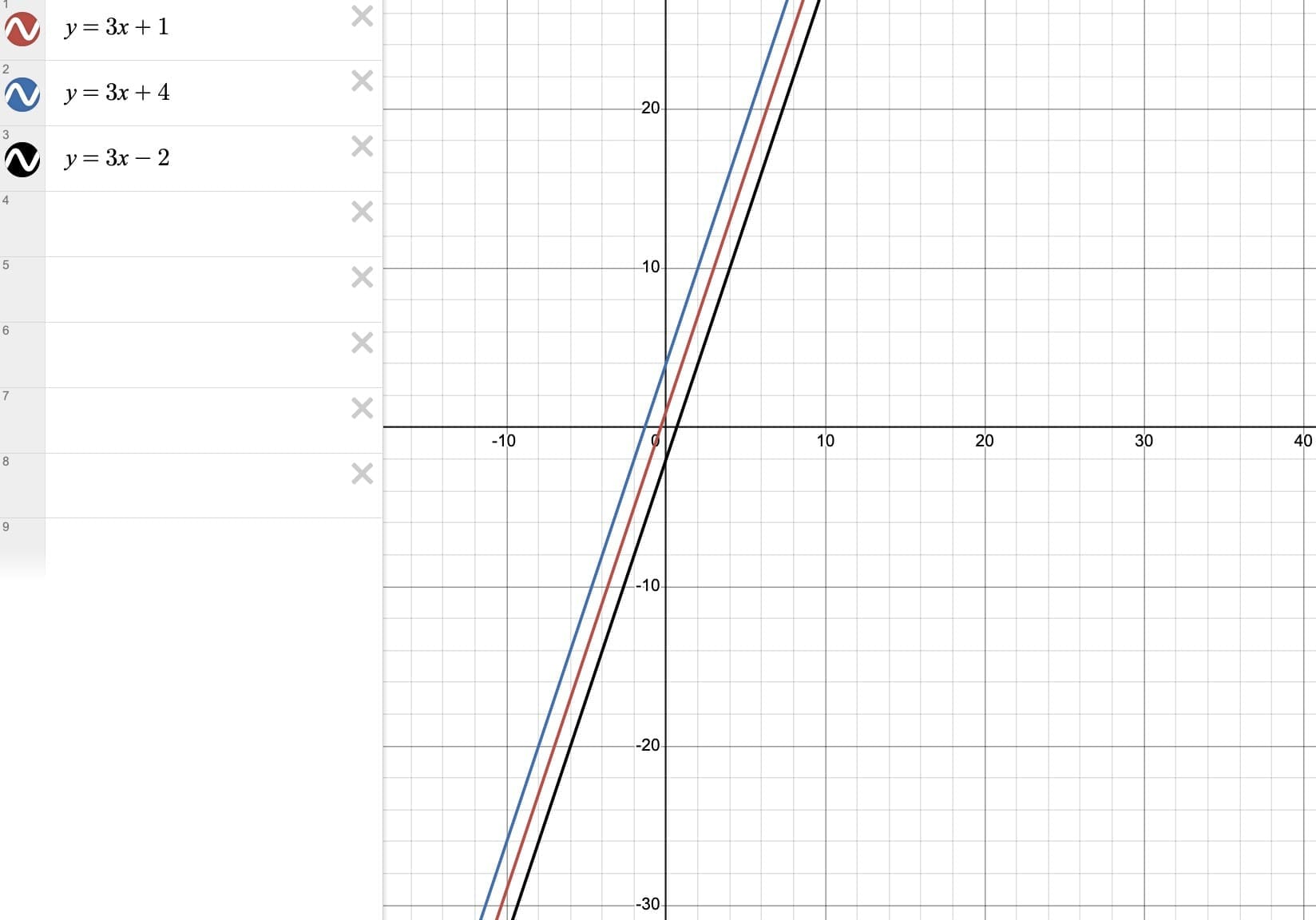
In y = ax + b, b is the y-intercept, where the line cuts the y-axis. Changing b shifts the line up or down but keeps slope same.
Example: 

Consider the equations:
y = 3x + 1, y = 3x + 4, and y = 3x – 2

In all equations, the slope a = 3 is the same, but the value of b is different.

For y = 3x + 1 → y-intercept = 1 → line cuts y-axis at (0, 1)
For y = 3x + 4 → y-intercept = 4 → line cuts y-axis at (0, 4)
For y = 3x – 2 → y-intercept = -2 → line cuts y-axis at (0, -2)

All lines have the same slope, so they are parallel. The line y = 3x + 4 is shifted upward, while y = 3x – 2 is shifted downward compared to y = 3x + 1.

8. Parallel Lines
Lines with the same slope (same a) but different b values are parallel.
Example: y = 2x + 1(red) and y = 2x + 5 (purple) are parallel lines.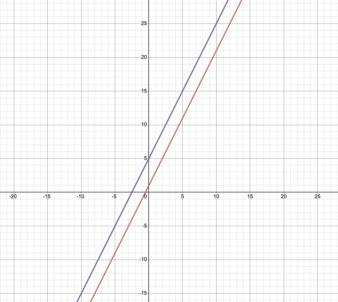

Key conclusions from graphing y=ax+b:

• a = slope: Controls steepness. When |a| > 1, line is steeper; when |a| < 1, line is flatter.
• b = y-intercept: The line crosses the y-axis at point (0, b).
• Lines of the form $y=ax$ (b = 0) always pass through the origin.
• Lines with the same slope (a) but different y-intercepts (b) are parallel.
• Changing b while keeping a fixed shifts the line up or down without changing its angle.
• Positive slope → linear growth; Negative slope → linear decay.

Summary

• An algebraic expression is made by combining numbers, variables, and operation symbols. For example, 2x² + 5xy – 3y² is an algebraic expression in variables x and y. The parts 2x², 5xy, and -3y² are called terms, and the numbers 2, 5, and -3 are called coefficients.
• Univariate polynomials are algebraic expressions that have only one variable. For example, x² + 5x + 3 and 3y³ – 4y² + 5 are univariate polynomials in x and y respectively. The highest power of the variable in a polynomial is called its degree. So, x² + 5x + 3 has degree 2 and 3y³ – 4y² + 5 has degree 3.
• A polynomial of degree one is called a linear polynomial. For example, 2x + 3 and 5 – 4y are linear polynomials.
• Linear growth means a quantity increases by a fixed amount over equal intervals. Linear decay means a quantity decreases by a fixed amount over equal intervals.
• A linear pattern is a sequence in which the difference between consecutive terms is constant.
• A linear relationship between two variables x and y is written as y = ax + b, which represents a straight line. Here, a is the slope and b is the y-intercept, which shows where the line cuts the y-axis. When b = 0, the equation becomes y = ax and the line passes through the origin.
• Linear growth is shown by a straight line with positive slope, while linear decay is shown by a straight line with negative slope.
• Parallel lines are of the form y = ax + b, where the slope a is the same but the y-intercept b is different.